Barotropic Model

This example is reworked from the original PyQG Barotropic Model example. We reproduce a plot from the paper “The emergence of isolated coherent vortices in turbulent flow” and illustrate the use of the BTModel as well as some more advanced diagnostics computations.

%env JAX_ENABLE_X64=True
import operator
import functools
import math
import matplotlib.pyplot as plt
import jax
import jax.numpy as jnp
import powerpax
import pyqg_jax

env: JAX_ENABLE_X64=True

Construct the Model

We will use a BTModel operating on a square \(2\pi\times2\pi\) periodic grid. We also configure the AB3Stepper to match the stepping used in PyQG.

DT = 0.001
T_MAX = 40
MEASURE_INTERVAL = 1
SNAP_INTERVAL = 5

stepped_model = pyqg_jax.steppers.SteppedModel(
    pyqg_jax.bt_model.BTModel(
        L=2 * jnp.pi,
        nx=256,
        beta=0,
        H=1,
        rek=0,
        rd=None,
        precision=pyqg_jax.state.Precision.SINGLE,
    ),
    pyqg_jax.steppers.AB3Stepper(DT),
)

stepped_model

SteppedModel(
  model=BTModel(
    nx=256,
    ny=256,
    L=6.283185307179586,
    W=6.283185307179586,
    rek=0,
    filterfac=23.6,
    f=None,
    g=9.81,
    beta=0,
    rd=0.0,
    H=1,
    U=0.0,
    precision=<Precision.SINGLE: 1>,
  ),
  stepper=AB3Stepper(dt=0.001),
)

Configure Initial Condition

The initial condition is randomized, we use a fixed seed for this example.

rng = jax.random.key(0)

The initial condition is generated with spectrum

\[ \big|\hat{\psi}\big|^2 = A\kappa^{-1}\bigg[1 + \Big(\frac{\kappa}{6}\Big)^4\bigg]^{-1}\]

where \(\kappa\) is the wave number magnitude. The constant \(A\) is chosen so the initial energy is \(\text{KE} = 0.5\).

# Compute ckappa base
ckappa = jnp.reciprocal(
    jnp.sqrt(
        stepped_model.model.wv2 * (1 + (stepped_model.model.wv2 / 36) ** 2)
    )
)
ckappa = ckappa.at[0, 0].set(0)

# Split RNGs and initialize pi_hat with noise
rng, rng1, rng2 = jax.random.split(rng, 3)
dummy_state = stepped_model.model.create_initial_state(jax.random.key(0))
pi_hat = (
    jax.random.normal(rng1, shape=dummy_state.qh.shape[1:], dtype=dummy_state.q.dtype) * ckappa
    + 1j * jax.random.normal(rng2, shape=dummy_state.qh.shape[1:], dtype=dummy_state.q.dtype) * ckappa
)
# Normalize values (zero mean and adjust KE)
pi = jnp.fft.irfftn(pi_hat, axes=(-2, -1))
pi = pi - jnp.mean(pi)
pi_hat = jnp.fft.rfftn(pi, axes=(-2, -1))
ke_aux = jnp.var(
    jnp.fft.irfftn(stepped_model.model.wv * pi_hat, axes=(-2, -1))
)
pih = pi_hat / jnp.sqrt(ke_aux)
qih = -stepped_model.model.wv2 * pih

# Package state for stepped_model
init_state = stepped_model.initialize_stepper_state(
    dummy_state.update(qh=jnp.expand_dims(qih, 0))
)

init_state

AB3State(
  t=f32[],
  tc=u32[],
  state=PseudoSpectralState(qh=c64[1,256,129]),
)

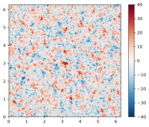
We can examine the initial state

vmax = 40
plt.imshow(
    init_state.state.q[0],
    vmin=-vmax,
    vmax=vmax,
    cmap="RdBu_r",
    extent=(0, stepped_model.model.W, 0, stepped_model.model.L),
)
plt.colorbar()

<matplotlib.colorbar.Colorbar at 0x7398746d6ba0>

Run the Model

We follow the example from Basic Time Stepping to roll out the trajectory using powerpax.sliced_scan() to skip steps according to MEASURE_INTERVAL.

@functools.partial(jax.jit, static_argnames=["num_steps", "subsample"])
def roll_out_state(state, num_steps, subsample):
    def loop_fn(carry, _x):
        current_state = carry
        next_state = stepped_model.step_model(current_state)
        return next_state, current_state

    _final_carry, traj_steps = powerpax.sliced_scan(
        loop_fn, state, None, length=num_steps, step=subsample,
    )
    return traj_steps

Before running the model we calculate the total number of steps we need to run as well as the subsampling we should apply before calculating diagnostics.

num_steps = math.ceil(T_MAX / DT) + 1
avg_subsample = math.ceil(MEASURE_INTERVAL / DT)

print(f"Total steps to run: {num_steps}")
print(f"Subsample factor for diagnostics: {avg_subsample}")

Total steps to run: 40001
Subsample factor for diagnostics: 1000

Roll out the trajectory for the above number of steps. Note that after generating, we drop the first state since this is the initial condition and it will significantly impact the spectra we will plot later. We do this using jax.tree.map() and operator.itemgetter() with an appropriate slice.

traj = roll_out_state(init_state, num_steps, avg_subsample)

# Skip the first (initial condition step)
# This does a slice of [1:] on each array
traj = jax.tree.map(operator.itemgetter(slice(1, None, None)), traj)

traj

AB3State(
  t=f32[40],
  tc=u32[40],
  state=PseudoSpectralState(qh=c64[40,1,256,129]),
)

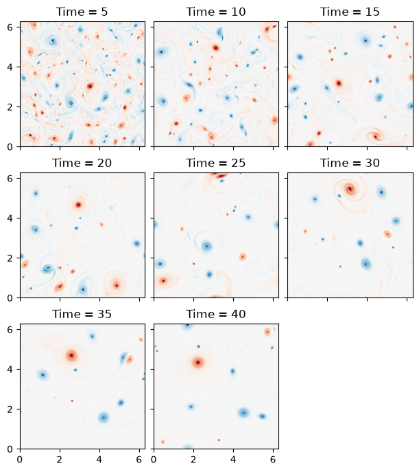
Plot States

We plot each snapshot, one for each SNAP_INTERVAL steps subsampled further from the diagnostic trajectory.

# Calculate the subsampling interval as well as how many rows, cols we need
plot_subsample_factor = math.ceil(SNAP_INTERVAL / MEASURE_INTERVAL)
cols = 3
rows = math.ceil(traj.t[::plot_subsample_factor].shape[0] / cols)
vmax = 40

fig, axs = plt.subplots(
    rows,
    cols,
    layout="constrained",
    figsize=(6, 2.25 * rows),
    sharex=True,
    sharey=True,
)

for raw_step_i, ax in enumerate(axs.ravel()):
    step_i = (raw_step_i + 1) * plot_subsample_factor - 1
    if step_i >= traj.tc.shape[0]:
        fig.delaxes(ax)
        continue
    step = jax.tree.map(operator.itemgetter(step_i), traj)
    ax.imshow(
        step.state.q[0],
        vmin=-vmax,
        vmax=vmax,
        cmap="RdBu_r",
        extent=(0, stepped_model.model.W, 0, stepped_model.model.L),
    )
    ax.set_title(f"Time = {round(step.t.item())}")

Diagnostics

Next we compute several diagnostics over this trajectory these use functions from the diagnostics module and most of the below calculations are patterned after the Diagnostics Example. However, the KE spectrum calculations have been modified significantly to illustrate changes in the spectra over time.

CFL

We begin by computing the CFL condition values. See pyqg_jax.diagnostics.cfl(). We report the worst CFL value and the average over the sampled states.

def compute_cfl(state, model, dt):
    full_state = model.get_full_state(state)
    cfl = pyqg_jax.diagnostics.cfl(
        full_state=full_state,
        grid=model.get_grid(),
        ubg=model.Ubg,
        dt=dt,
    )
    return jnp.max(cfl)

@jax.jit
def vectorized_cfl(traj, stepped_model):
    return powerpax.chunked_vmap(
        functools.partial(
            compute_cfl, model=stepped_model.model, dt=stepped_model.stepper.dt
        ),
        chunk_size=100,
    )(traj)

traj_cfl = vectorized_cfl(traj.state, stepped_model)

print(f"Max CFL: {jnp.max(traj_cfl)}")
print(f"Avg CFL: {jnp.mean(traj_cfl)}")

Max CFL: 0.19400572776794434
Avg CFL: 0.1468898355960846

Kinetic Energy

We calculate the total KE in each snapshot taken in the trajectory. See pyqg_jax.diagnostics.total_ke().

def compute_ke(state, model):
    full_state = model.get_full_state(state)
    return pyqg_jax.diagnostics.total_ke(full_state, model.get_grid())

@jax.jit
def vectorized_ke(traj, model):
    return powerpax.chunked_vmap(
        functools.partial(compute_ke, model=model), chunk_size=100
    )(traj)

traj_ke = vectorized_ke(traj.state, stepped_model.model)

print(f"Max KE: {jnp.max(traj_ke)}")
print(f"Min KE: {jnp.min(traj_ke)}")

Max KE: 0.4965575337409973
Min KE: 0.49244457483291626

Note that kinetic energy is nearly conserved over the course of the run.

Kinetic Energy Spectrum

The KE spectrum calculations are the most heavily modified from the templates provided in the Diagnostics Example document. Instead of calculating one spectrum over the entire trajectory, we use additional JAX transforms to calculate multiple spectra over disjoint time intervals. This is relatively straightforward since in the JAX port, diagnostics are computed after the simulation run so the bins for averaging can be adjusted after the snapshots are gathered.

The chunked_ke_spec function below divides the trajectory into chunks of KE_SPEC_CHUNK_SIZE snapshots. This is in addition to the subsampling done while generating the trajectory. That is, each chunk is over a time range of KE_SPEC_CHUNK_SIZE * MEASURE_INTERVAL.

KE_SPEC_CHUNK_SIZE = 10

def compute_ke_spec_vals(state, model):
    full_state = model.get_full_state(state)
    ke_spec_vals = pyqg_jax.diagnostics.ke_spec_vals(
        full_state=full_state,
        grid=model.get_grid(),
    )
    return ke_spec_vals

@functools.partial(jax.jit, static_argnames=["chunk_size"])
def chunked_ke_spec(traj, model, chunk_size):
    # If the trajectory is not evenly divisible by chunk_size
    # we need to remove trailing elements
    chunk_size = operator.index(chunk_size)
    if chunk_size < 1:
        raise ValueError(f"chunk_size must be at least 1 (got {chunk_size})")
    traj_len = jax.tree.leaves(traj)[0].shape[0]
    num_chunks = traj_len // chunk_size
    # Remove any trailing steps to traj evenly splits into chunks
    traj = jax.tree.map(
        operator.itemgetter(slice(None, num_chunks * chunk_size)),
        traj,
    )
    # Compute the ke_spec_vals over the trajectory as usual
    traj_ke_spec_vals = powerpax.chunked_vmap(
        functools.partial(compute_ke_spec_vals, model=stepped_model.model),
        chunk_size=100,
    )(traj)
    # Break the spectral values into chunks and average within each chunk
    traj_ke_spec_vals = traj_ke_spec_vals.reshape(
        (num_chunks, chunk_size) + traj_ke_spec_vals.shape[1:]
    )
    ke_spec_vals = jnp.mean(traj_ke_spec_vals, axis=1)
    # Compute the spectrum over each chunk separately
    # Use in_axes to avoid vmapping over the model grid
    ispec = jax.vmap(pyqg_jax.diagnostics.calc_ispec, in_axes=(0, None))(
        ke_spec_vals, model.get_grid()
    )
    # Each spectrum has the same ispec_grid, these are not vectorized
    kr, keep = pyqg_jax.diagnostics.ispec_grid(model.get_grid())
    return ispec, kr, keep

traj_ke_spec, kr, keep = chunked_ke_spec(traj.state, stepped_model.model, KE_SPEC_CHUNK_SIZE)

We plot each spectrum separately on the same axes with two dotted trendlines.

for i, tks in enumerate(traj_ke_spec):
    min_time = KE_SPEC_CHUNK_SIZE * i * MEASURE_INTERVAL
    max_time = KE_SPEC_CHUNK_SIZE * (i + 1) * MEASURE_INTERVAL
    plt.loglog(kr[:keep], tks[0, :keep], label=fr"$\text{{time}} \in ({min_time}, {max_time}]$")
plt.xlabel("Wavenumber ($k$)")
plt.ylabel("KE")
plt.ylim(1e-10, 1)
plt.grid()
plt.legend()

ks = jnp.array([3.0, 80.0])
mid_k = 10**(jnp.mean(jnp.log10(ks)))
for i, (y_off, slope) in enumerate([(4, -4), (20, -3)]):
    es = y_off * ks**slope
    midpt = y_off * mid_k**slope
    plt.loglog(ks, es, "k--")
    plt.text(
        mid_k,
        midpt,
        fr"$k^{{{slope}}}$",
        fontsize="large",
        horizontalalignment="left" if i == 1 else "right",
        verticalalignment="bottom" if i == 1 else "top",
    )

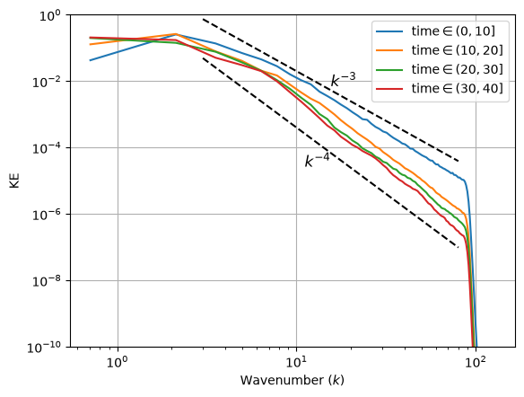
Note how—as in the McWilliams paper—the spectrum becomes steeper over time.

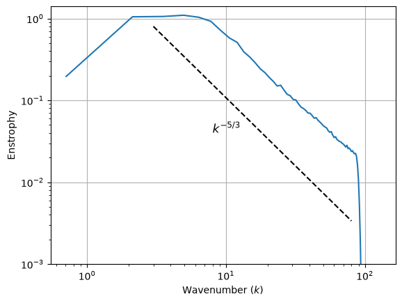
Enstrophy Spectrum

We calculate the enstrophy spectrum for the entire trajectory (see pyqg_jax.diagnostics.ens_spec_vals())

def compute_ens_spec_vals(state, model):
    full_state = model.get_full_state(state)
    e_spec_vals = pyqg_jax.diagnostics.ens_spec_vals(
        full_state=full_state,
        grid=model.get_grid(),
    )
    return e_spec_vals

@jax.jit
def vectorized_ens_spec(traj, model):
    traj_ens_spec_vals = powerpax.chunked_vmap(
        functools.partial(compute_ens_spec_vals, model=stepped_model.model),
        chunk_size=100,
    )(traj)
    ens_spec_vals = jnp.mean(traj_ens_spec_vals, axis=0)
    ispec = pyqg_jax.diagnostics.calc_ispec(ens_spec_vals, model.get_grid())
    kr, keep = pyqg_jax.diagnostics.ispec_grid(model.get_grid())
    return ispec, kr, keep

traj_ens_spec, kr, keep = vectorized_ens_spec(traj.state, stepped_model.model)

and plot it with a dashed trendline.

ks = jnp.array([3.0, 80.0])
es = 5 * ks**(-5/3)
plt.loglog(kr[:keep], traj_ens_spec[0, :keep])
plt.loglog(ks, es, "k--")
plt.text(8, 0.04, "$k^{-5/3}$", fontsize="large")
plt.xlabel("Wavenumber ($k$)")
plt.ylabel("Enstrophy")
plt.ylim(1e-3, 1.4e0)
plt.grid()