Surface Quasi-Geostrophic (SQG) Vortex

This example is reworked from the original PyQG SQG example. We reproduce a plot from the paper “Surface quasi-geostrophic dynamics”.

import operator
import functools
import math
import matplotlib.pyplot as plt
import jax
import jax.numpy as jnp
import powerpax
import pyqg_jax

Construct the Model

We construct the SQGModel object with adjusted parameters, and wrap it in a stepper for later simulation.

DT = 0.005
T_MAX = 8
SNAP_INTERVAL = 2

stepped_model = pyqg_jax.steppers.SteppedModel(
    pyqg_jax.sqg_model.SQGModel(
        L=2 * jnp.pi,
        nx=512,
        beta=0,
        Nb=1,
        H=1,
        f_0=1,
    ),
    pyqg_jax.steppers.AB3Stepper(dt=DT),
)

stepped_model

SteppedModel(
  model=SQGModel(
    nx=512,
    ny=512,
    L=6.283185307179586,
    W=6.283185307179586,
    rek=5.787e-07,
    filterfac=23.6,
    f=None,
    g=9.81,
    beta=0,
    Nb=1,
    f_0=1,
    H=1,
    U=0.0,
    precision=<Precision.SINGLE: 1>,
  ),
  stepper=AB3Stepper(dt=0.005),
)

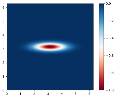
Configure Initial Condition

The initial condition in this example is an elliptical vortex

\[ -\alpha\exp\bigg(\!-\frac{x^2 + (4y)^2}{(L / 6)^2}\bigg) \]

The amplitude is \(\alpha = 1\) which sets the strength and speed of the vortex. The aspect ratio in this example is 4 and gives rise to an instability.

We calculate the values for this initial condition

x = stepped_model.model.x - jnp.pi
y = stepped_model.model.y - jnp.pi
vortex = -jnp.exp(-(x**2 + (4 * y) ** 2)/( stepped_model.model.L / 6) ** 2)

We can examine the initial state

plt.imshow(
    vortex,
    cmap="RdBu",
    vmin=-1,
    vmax=0,
    extent=(0, stepped_model.model.W, 0, stepped_model.model.L),
)
plt.colorbar()

<matplotlib.colorbar.Colorbar at 0x785635faa510>

and finally package it into a stepped state object

init_state = stepped_model.create_initial_state(jax.random.key(0)).update(
    state=stepped_model.model.create_initial_state(jax.random.key(0)).update(
        q=jnp.expand_dims(vortex, 0)
    ),
)

init_state

AB3State(
  t=f32[],
  tc=u32[],
  state=PseudoSpectralState(qh=c64[1,512,257]),
)

Run the Model

We roll out the initial state up to T_MAX taking snapshots according to SNAP_INTERVAL.

@functools.partial(jax.jit, static_argnames=["num_steps", "subsample"])
def roll_out_state(state, num_steps, subsample):
    def loop_fn(carry, _x):
        current_state = carry
        next_state = stepped_model.step_model(current_state)
        return next_state, current_state

    _final_carry, traj_steps = powerpax.sliced_scan(
        loop_fn, state, None, length=num_steps, step=subsample,
    )
    return traj_steps

Note the use of powerpax.sliced_scan() above to skip steps between each snapshot. This produces a trajectory traj that we can examine.

num_steps = math.ceil(T_MAX / DT) + 1
snap_subsample = math.ceil(SNAP_INTERVAL / DT)

traj = roll_out_state(init_state, num_steps, snap_subsample)

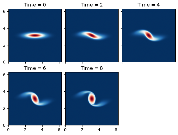
Plot States

We plot each of the snapshots taken from the simulation. With access to more time (or ideally a GPU) this model can be simulated for a longer time period by adjusting T_MAX above.

cols = 3
rows = math.ceil(traj.tc.shape[0] / 3)
fig, axs = plt.subplots(
    rows,
    cols,
    layout="constrained",
    figsize=(6, 2.25 * rows),
    sharex=True,
    sharey=True,
)

for step_i, ax in enumerate(axs.ravel()):
    if step_i >= traj.tc.shape[0]:
        fig.delaxes(ax)
        continue
    step = jax.tree.map(operator.itemgetter(step_i), traj)
    data = step.state.q[0]
    ax.imshow(
        data,
        vmin=-1,
        vmax=0,
        cmap="RdBu",
        extent=(0, stepped_model.model.W, 0, stepped_model.model.L),
    )
    ax.set_title(f"Time = {step.t.item():.0f}")